Transcript
- Transcript — Transcript – Briggs, 2015 – The Crisis Of Evidence, Or, Why Probability & Statistics Cannot Discover Cause – YouTube
<aside> 💡 So basically what I want to tell you is that probability and statistics cannot do what they promise to do, in its classical sense, and that’s to show causation.
</aside>
<aside> 💡 And that’s the philosophical topic. And I want to explain that first, and then I’m going to show you that even if we assume that probability and statistics can show causation, even if we do understand causation, the procedures that we use are wrong and they should be adjusted and done in a completely different way.
And that way is essentially just what Ed was telling us. We replicate, we replicate. We have a model, we make predictions. We see if those predictions are upheld, and we have to do that repeatedly.
The problem with probability and statistics is they seem to show us, give a shortcut. They seem to promise that we could know things with very little effort. And I’m going to prove that to you.
</aside>
<aside> 💡 So what are traditionally probability and statistics used for? What do you think they’re used for?
Explain or quantify uncertainty in that which we do not know. And nothing else.
</aside>
<aside> 💡 Strangely, however, classical procedure in both its frequentist and Bayesian procedures, say the opposite.
</aside>
So let me give you a little example.
in a low or no group of 1,000 5 people got cancer of the albondigas, and in the “some” or high PM2.5 group of 1,000 15 did
<aside> 💡 What is the probability that more people in the High Group had cancer? One. That’s it. So I’ve proved to you that we do not need probability and statistical models to tell us what we already know. We do not need any other kind of model.
</aside>
<aside> 💡 We can say that there’s three times as many people got sick in the High Group, or only five people got sick in the Low Group. We know these things by observation. We do not need probability and statistics to tell us what we’ve already seen.
</aside>
But what are the real questions of interest here?
<aside> 💡 Why do you do a statistical study like this? What caused the difference? That’s the first.
</aside>
<aside> 💡 Speaker1: [00:04:32]
But no matter what, something caused each of those cancers. We want to know, can probability and statistics answer that question? And the the answer to that is no. Although everybody assumes it does.
</aside>
<aside> 💡 The second question that probability and statistics can answer is: Given that I assume I do know the cause, which I cannot learn from probability and statistics – some other way I learn it. But assuming I do know the cause, what can I say about future groups of people who are exposed or not? What can I say about the uncertainty in their cancer rates? That’s where probability and statistics can be useful.
</aside>
So what is probability and statistics answer to causality?
How do we typically do a statistical procedure in this type of a case?
Some sort of hypothesis test, correct?
<aside> 💡 Step one is always the same, and that is always to form some sort of usually parameterized probability model for the observed data.
</aside>
<aside> 💡 Step two is to form what we call the null hypothesis.
</aside>
<aside> 💡 Now, we already know that that’s false.
Did we not say there’s 100% probability the groups are different? Yes. So why do we want now?
Why do a null hypothesis test? We’ve already ascertained the groups are in fact different. 100% certain.
</aside>
<aside> 💡 Number three is the calculate a statistic.
A statistic is just a function of the data. Many statistics are available, hence the field statistics.
</aside>
<aside> 💡 Step four is to calculate this creature (p-value):
Given the data we’ve assumed, given the model we’ve assumed, given the data we’ve observed, and assuming the null hypothesis is true, we calculate the probability of seeing a test statistic larger than the one we actually got, in absolute value, assuming we could repeat the experiment an infinite number of times. This is called the p value.
</aside>
The P value for this particular data happens to be for a test of so called differences in proportions, .04. So what do we say?
.04 is less than the magic number. The number is Magic. Gigerenzer, Another critic of the field of statistics, calls this procedure ritual. Zizek [sp?tk] calls it something I can’t repeat. I call it magic. It is the magic number.
<aside> 💡 If the P value is less than the magic number. You have success. You have statistical significance. You can write grants, you can write your papers. It will be accepted and all this kind of glorious things.
</aside>
<aside> 💡 What does p-value mean?
Given the model we’ve assumed, given the data we’ve seen, accepting the null hypothesis is true. It’s calculating the probability of a test statistic larger than the one we actually got in absolute value if we were to repeat the experiment an infinite number of times. And that’s all it means.
It certainly does not say anything about cause.
It does not say in this p value is less than the magic number. But it does not then prove that PM2.5 is a cause of the cancer of those people in the High Group.
</aside>
<aside> 💡 If we assume PM 2.5 as a cause. If we don’t know it’s a cause, then we don’t know what caused the cancer of the people in the low group. And we also don’t know what caused the cancer and the people in the High Group.
</aside>
But if it is a cause, it is always a cause. Unless it is blocked. And the other option is. It is not a cause, as simple as that.
BK: “blocked” can mean confounding (but it can work both ways – it not only blocks the cause but it may yield a false positive cause)
<aside> 💡 So it’s either always a cause, it is a cause or it isn’t. A cause is a tautology.
That statement is true. I can say that chewing on pencils is or isn’t a cause of cancer of the abundance. That is a true statement.
I can say that wearing hats is or isn’t a cause of cancer of the albondigas because that is a true statement. It is a true statement because it is a tautology.
Tautology. These are always true. Therefore, it adds nothing to the logic of the situation.
Merely proposing a cause does not prove in any way that it is a cause or give any extra probability to the idea that it’s a cause.
That is a very subtle but difficult point.
If you can understand that, you can understand the real deep hole that probability and statistics have dug themselves. Because they do say that you can ascertain the probability that it’s a cause. But it’s not true.
</aside>
Here’s the second point. Now, on any given person or group of people, we can measure innumerable things, not infinite, but large.
Now it’s almost certain to be true that in these groups, these two groups, this low in this high group, there will be other differences that only apply to the high people and the low people.
<aside> 💡 Speaker1: [00:13:05] Now I said that the two groups were high and low PM 2.5 and I did this statistical test and I got statistical significance. And that led me to say that PM 2.5 is associated with or linked to or causes the cancer. But then it’s an arbitrary label.
I could have just as easily put low and high bananas.
This is also true of these people that I’ve measured.
Everybody in the low group had one fewer banana. Therefore, I also have to say that the p value that I got also proves that bananas are a cause of the cancer. And that’s true of every other thing that’s different between these two groups. And that’s absurd.
</aside>
**As the number of UFO reports increased, so did the temperature anomaly. Now we all laugh at that. If he had statistics, p values, all this kind of thing and the usual hypothesis test and we laugh at that. But why? Why are we laughing at that? Why is it absurd?
That’s because we understand the essence of the situation.
It’s absurd. It’s nuts.**
We understand what’s going on with the temperature and we know it cannot have any causative play with these fictional UFO observations. We understand yet every statistical test it passed in glory. Yet we’re willing to say that PM 2.5 might be a cause of cancer and not the bananas, because we’re trying to get at something else that we cannot get from these statistical procedures. And this is the idea of essence.
And the philosophical system that Ruled Most people for the greater part of the 20th century was something called empiricism.
<aside> 💡 But let me lead you to a little bit of the background on this strange idea that probability and statistics can show cause.
</aside>
So imagine instead of 15 people in the High Group. Having cancer, it was only 14. The P value is now 0.06. What do we say? It’s not significant.
What else can we say? Chance.
Yes, we’re saying that chance caused the results. There is no such thing.
There is no such thing as chance. Chance is an epistemological state. It’s a state of our knowledge.
There is no such thing as a material chance.
There is no energy called chance.
There is no force called chance nor randomness.
Chance or randomness cannot be a cause.
It’s impossible that it could be a cause, something physical or biological, I should say, or some combination, caused each of these cancers. It cannot have been chance.
Chance and randomness are a product of our epistemology, of our state of knowledge. They basically mean, I don’t know what caused these things.
So that’s fair enough.
I could say I don’t know what caused these Things But because if I just add one more person with cancer, I all of a sudden say the cause is definitely PM 2.5. That’s a fallacy.
Figure. Let’s play: Who Said It!

- David Hume
- Karl Popper
- Karl Popper
- Karl Popper
It was Hume’s idea that we can never really observe or understand cause. We can only look at events. This event followed by that event, everything is entirely loose and separate.
But the next man who is responsible for the next three quotes, Karl Popper did, he was a logical positivist, not quite part of the Vienna circle, but one of their associate members.
Popper believed in this idea called falsifiability.
Perhaps you’ve heard of this science.
**Scientific theory is not a scientific theory unless it is falsifiable.
He said that unless you can prove something that is false, it’s not scientific. Empirically prove, meaning with observation.**
Now logical positivism said, you can never believe any theory except based on empirical evidence. Should we believe logical positivism then, because that’s not empirically provable. And so basically logical positivism died out in the 20th century.
David Stove, a philosopher from Australia, basically called it an episode in black comedy.
But this idea of poppers became exceedingly popular among scientists. We hear this all the time. That’s not falsifiable. Not falsifiable. So it isn’t scientific. Well, it was very influential with RA Fisher. He’s sort of the father of modern day frequentist statistics.
It was Fisher that developed the p value. He loved this idea of poppers that you could never believe anything but you could disbelieve. And he wanted to build falsifiability into the practice of probability and statistics. So he developed this p value.
He said once the p value is less than the magic number. He didn’t use the word magic number. But **once the p value is smaller than something, you are then allowed to say that the null hypothesis is false.
You are allowed to act as if it is false.
You are allowed to believe it is false.
Now, this is a pure act of will.
You’ve not proven anything false. You haven’t come up with a probability that anything is true or false. It is a pure act of will.**
And that was Neyman and Pearson’s criticism of the P value, there were other statisticians early in the 20th century who said don’t use the P value because it will lead you to make these kind of mistakes that everybody is now making. Now the fields are inundated with this kind of thinking, especially in fields like sociology, psychology, and even in medicine.
These PM 2.50, in medicine and so forth that use p values statistical significance as the proof that I have discovered cause and we’ve already seen that can’t be true.
Now, if the p value is greater than the magic number we say we fail to reject. Right. We don’t say we actually accept the null. And that’s because of Karl Popper. We failed to reject because we’re only always after rejecting, because when we reject something, we falsified.
But it’s just as nonsensical because if we take a proposition and say we could never believe any proposition. We can only believe that we have proved it false. That means we’re believing a proposition just like this last thing here. It’s self refuting.
p values are self refuting. In fact, you can show in an argument which I won’t do here, they add nothing. They add no information to the problem at all.
P values were always an act of will.
This is why we need to do something else. We need to look at essence.
Ed showed us this morning when he was first doing his experiment, his advisor asked him to do and redo and redo and redo.
All work like this, all real scientific labor, as we all know when we’re involved in studies, is extremely laborious, difficult, hard work.
But statistics promises that we could do it in an instant. All we have to do is submit this data to some test.
Q: Are you dismissing Karl Popper?
Yes, I am.
Math, for instance, no mathematical proposition can be falsified. Any theorem that we have proved true cannot be falsified. No empirical evidence can ever show a mathematical theorem to be false.
Probability is not falsifiability, for the most part.
Many people use normal distributions and regression and so forth. What’s the extent of a normal distribution? What does it give probability to? If I can ask the experts in the audience: anywhere from negative infinity to infinity, so that any observation we make will never falsify a probability statement. That’s why you have to say “practically falsified.”
But that has the same epistemic status as “practically a virgin.” It’s an act of will. It doesn’t have anything to do with anything else.
Now, if I had a pencil here, I could do this. So let me do this. Let me this. Talk about the essence thing. So what I’m going to do is I’m going to let go of this. What’s going to happen?
It’s going to fall.
Why do we need a statistical test? No, we understand gravity.
We various levels of understanding of gravity exist at some high level. We understand it’s the nature of gravity, the mass of this thing and the mass of the earth to bend space.
But we also understand it’s the power of gravity to cause things to fall. It’s not because some equation exists out there, some instrumentalist equation.
Quantification is very nice and when we can quantify things, but not everything can be quantified.
Even if we do understand cause. Which sometimes we do. Even more. We don’t need to use probability and statistical models to tell us what cause might be.
Think about this. You’re at the casino. You’ve been playing roulette in the last ten times. It’s come up red. Is black due. Why not? It’s called the Gambler’s Fallacy. We all know that. Yes, but why is not black due? If we were to use the statistics, we’d have to say the p value is going to be one. It’s going to be P, it’s going to be two to the minus ten. It’s a very low number. There’s no probability. There’s no probability, as will something’s causing that ball to rattle around.
That’s the key, the cause. We all understand there’s nothing in the nature of the physics that have changed. It stayed the same. The wheel might have worn infinitesimally from one run to the next. That’s true, but we could move to other examples where there is no wearing of parts.
So what we need to do is understand cause we need to understand essence
But still, just by saying something is possibly a cause is no evidence of cause. It doesn’t give you anything. Anything could possibly be a cause. But we were trying to get at this nature of it. In order to find the real nature, we have to understand the etiology of the disease.
But in order to answer the real question, we have to not do the shortcut that probability and statistics seemingly provides us.
And I’m giving you the example in PM 2.5, but this must be done with absolutely every statistical analysis.
**See, what I call the epidemiologist fallacy is when an epidemiologist or statistician or doctor, if somebody says X causes Y, but where he never measures X, never measures X, and where he ascertains through statistical models that X is a cause.
Now the epidemic epidemiologist fallacy is a compound then of the ecological fallacy, which is when you don’t measure what you want to measure and instead measure a proxy and say the proxy is the same as the thing you want to measure. And the ascertaining of cause through probability models. I call it the epidemiologists fallacy.
Without the epidemiologists fallacy, epidemiologists would be out of work. They have these data sets, they go in and they just start playing around. They start looking for P values that are wee P values and they start publishing and this is nonsense.
So we need to understand first what we’re dealing with. All of the papers that I have discovered that have claimed a causative agency for PM 2.5 use the epidemiologists fallacy.**
You already know the facts, but he looked at the epidemiologist factor angle, which is to say all of these studies measure some kind of ambient PM 2.5, some average level. For instance, Los Angeles, they’ll measure the PM, the average level of PM 2.5 in Los Angeles and then ascribe that to every single person in their study, which is nonsense.
There are several studies that don’t show any statistical significance, and these are the ones, just as Ed says, the regulators leave out.
There’s a Seventh Day Adventist study. You’ve heard of the six cities. Willie showed it in the American Cancer Society study.
I’m about to show you these predictive methods. And I applied. Jim, help me out on this to get the data from the ACS. They claim that they’ll let researchers have it if they can show a good reason for it. I applied in the normal process and showed them my bona fides, all this kind of thing, and I was rejected. So they actually, like everybody else, don’t want to know how bad things are. But I did them on my own anyway.
**But the risk ratio for going just 20 micrograms above baseline PM 2.5, anywhere from 1 to 10 was about 1.7, 1.17 and 1.7. So if you work that out, if you give the equivalent of the PM 2.5 as cigarette smoke, that means that PM 2.5 must be gamble proved about 150 to 300 times more toxic than smoking two packs of cigarettes a day for many years.
Speaker1: [00:37:25] So just going out and breathing the air outside here is more toxic for you than being a chain smoker. That’s what the results prove. So that’s why we need these predictive methods.**
Figure. Risk ratio

So risk ratio is a very common way to present results. Everybody thinks it’s just kosher as anything. It is extremely misleading. It’s a terrible way to show results, and I’m going to prove that to you.
It’s the probability of having the disease, the malady, whatever, given that you were exposed divided by the same probability, given you are not exposed.
**Well, risk ratio only applies to single people. It only applies to one individual at a time. And if you’re just one individual, you don’t care about the risk ratio. You care about these individual probabilities.
If I’m not exposed, the probability is one in 10 million. If I am exposed, it’s two in 10 million.**
Speaker1: [00:40:15] So this is the way if you work out these numbers, the probability of at least one person getting it in the exposed group and at least one person getting the non exposed group works out to be this. **The risk ratio has suddenly dropped.
If you do it for New York City, which has LA, has about 4 million people, New York has eight. The risk ratio drops again to about 1.7. If you do it for the entire United States, the risk ratio drops to something just over one.**
Figure. Jerrett et al.

So here is the interesting one. Now this is the paper that I looked at in depth and my I wrote a bunch of I wrote an official comment on this and it was submitted to the California Air Resources Board at one of their meetings. Jim has actually the audiotape of or the MP three file or something in this and you can listen to their comments about my criticisms.
And basically, I think I told this group before that they considered what I had to say and they basically said, well, you know, Dr. Briggs is right, but everybody else makes these same mistakes. Therefore, We don’t want to be different. I’m not kidding.
So two in 10,000 is more than regulation worthy, according to the EPA. I got this directive that’s well within their bounds for considering a government action.
You know, EPA agents now are armed, right? They carry weapons. Some of these guys, they go out in the field when they’re testing things. So they’re dead serious about these things.
Now, it turns out that Jerrett’s risk ratio 1.06, if we use this two times ten to the minus for the two and 10,000 watermark, that works out to be 1.89. That’s the probability of having the disease or morbidity for the not exposed group.
Now, let’s apply this to Los Angeles.
We need to apply this. It just doesn’t make any difference. Yes, this 1.06 had a small p value. Yes, he did in fact use the epidemiologist fallacy. He used this land use regression model to guess exposure. He never measured exposure on anybody, ever. Nobody did. It’s just Wild. It’s nonsense is what it is.
Figure. Probabilities of developing cancer

Now, these are not normal distributions. They kind of look at their binomial because remember, we’re assuming these numbers are true. We’re assuming that this is the best case in their world. What I have here is this dash group, the middle one, this dash one right here. These are the 2 million people. I’m I’m basically assuming here I don’t have anything else I could do, that half the people in LA did not get exposed and half the people did.
To this high level of PM 2.5. Basically there’s a 99.99% chance that 330 to about 450 people will get cancer in the low group in the people who weren’t exposed with about 380 being the most likely number and about 400 people and the people who were exposed, that’s a difference of about 20 people.
So all of LA. The difference is about 20 people. That’s what I can expect. Even assuming there are things. So how much money would you pay to eliminate Pm 2.5? That’s too much. Because why?
Because we don’t know Pm 2.5 as a cause. This is assuming it’s a cause. We still don’t know. It’s a cause.
Figure. Probabilities of developing cancer, half exposed

This is the real curve to look at. This is now the dashed line is assuming all 4 million LA residents are not exposed. All 4 million residents are not exposed. It’s anywhere from like 680 people to about 800 and 850. There’s a 99.9% chance. That’s how many cancer cases we’ll see. That’s a predictive model. This is no. Speaker2: [00:45:37] Longer. Speaker1: [00:45:38] Confidence intervals or p values or any of this kind of stuff.
I’m saying given the information that I have, what’s the probability of stuff I don’t yet know? Which is the future. Now, given that half are exposed and half. Are not exposed This is the number of people we expect to see. This is without any regulation of PM 2.5 assuming PM 2.5 is a cause. And the difference is still just about 20 people and the maximum you could get if you take this point here and this point here, meaning the most worst situation you can imagine, a 99.9% chance of having 867 people or so having cancer if I didn’t do anything. And the worst case scenario here, meaning the best case scenario, meaning only like 690 people got cancer, is a savings of 200 lives. But the probability of that happening is only like 0.05.
The overwhelming probability is if you were to eliminate PM 2.5 completely. This is using Jarrett’s data from best I can tell eliminated completely. The best is the savings that you could expect of about 20 lives. The best.
But notice I just took his 1.06 from his paper and said, That’s it. Is that true, though? When we do a statistical model, are we certain of these estimates? Now, there’s some uncertainty in these estimates. There’s some plus or minus, and there’s various mathematical ways to deal with these uncertainties.
**The way I used and the way that I advocate everybody use I don’t have any time to explain this is to use the
Bayesian posterior predictive distribution.
In other words, I want to say what the future will be like integrating out all uncertainty I have in these mathematical parameters.**
So I’m going to basically take that 1.06 and the plus or minus whatever Jared had published. And I’m going to put that plus or minus in here and add the uncertainty. Okay. I’m going to add that on. I have to. I can’t just use the 1.06. That’s not fair.
That’s not even taking their published results seriously. I need to take that plus or minus into account.
Figure. Probabilities of developing cancer taking uncertainty into account

This is the result. This right here assumes this dash line that if I removed PM 2.5, all 4 million residents of LA would not be exposed. This is the number of, I guess its cardiac cases. I don’t know exactly what miss or something. Anywhere from 500 to 1000 people. There’s a 99% chance, 99.99% chance of that. However, if Half were exposed to PM 2.5 and half not The savings in lives now is about from the peak of this to the peak of this is two. Now, that should be stunning to you, but you’re not used to seeing statistics put in this way.
**But the difference the real difference, the real expected difference that we could see is trivial. And that’s assuming PM 2.5 as a cause we don’t know PM 2.5 is the cause so the real savings are much less. And if we factor in the epidemiologist fallacy, any purported savings disappear entirely.
And this is the way that all of these studies should be done. You cannot use hypothetical populations. You have to use real predictive methods that say nothing about all these parameters like P values and confidence intervals and all this nonsense. And you have to do it in this predictive way. You have to make real predictions.
Now, notice I’ve made a prediction or Jerrett has. What do I do next? I see if it’s true. I wait for data. This is what everybody else has to do. Why is it that when the model itself tells us the theory is desirable, that I’m removed from the responsibility of checking?
That happens in global warming. It happens for anything the government wants to regulate.**
So let me just recap here.
We did a lot what I wanted to show you. And I called this talk the crisis of evidence, because that’s exactly what it is, at least in medicine and these type of fields. They’re making a stab at understanding what the real causes are for these things.
**Everybody just keeps assuming the stuff and nobody checks.
I mean, it used to be in physics when you made things and if you’re an engineer, you have to check your stuff against reality.
So the way to do statistics is first try to understand like everybody does. The hard way. And if you’re not going to do that, at least do this in a predictive way then wait and see if your model has any damn value before proclaiming that it does.**
So it’s it’s not a panacea. There’s not saying that statistics is going to certainly provide us good models. And just like the chess example causes undetermined, we can’t tell from the data.
So we have to do a lot of hard work. If I’ve just given you a little bit of disquiet, that’s all I think I could do at this point. I have paper on this at archive.
Just look up my name and archive and you can read a fuller version of this. And that’s the rest of my contact information.
The Crisis Of Evidence: Why Probability And Statistics Cannot Discover Cause
Q: Question is, you said either it causes cancer or it doesn’t cause cancer. But my understanding was, I mean, sometimes we think **maybe it takes three things together to cause the cancer. So given that, isn’t it useful to to sort out confounding variables?
Speaker1:** [00:52:44] Yes, that’s what I say. So it’s either always a cause or it is sometimes blocked. It can be blocked by missing a catalyst, for instance. Yes, exactly right. But that was just a subtle philosophical point to show you that you cannot it’s like multiplying an algebraic equation by one, a tautology in logic. It doesn’t provide additional information, but finding all these things like Ed showed us, he had this, the cause was there, and they went and they did a counterfactual. They they block some pathway. And there was the block and and then the cause disappeared. So it’s just those kind of things.
BK: think about the oncogenic paradox and how there are many carcinogens…that damage mitochondrial respiration…which can lead to compensatory fermentation…and cancer
The mathematics works out beautifully, but deciding what to do based on a p value is an act of will. It’s it’s completely arbitrary. What you do with it is arbitrary in the extreme.
Mathematicians are weird, you know, I’m one of them and they don’t always come down to reality. They don’t understand how this stuff is going to apply in real life. And you can’t just because it’s an equation and you can match the terms in that to real life things doesn’t mean it works for those real life things. And that’s the problem.
Popper was wrong, but he had a very good motive. It’s the same thing. He basically was looking at UFOs and these kinds of things and homeopathy and the like, saying that any observation confirms the theory, these people said, And that’s exactly what we have at global warming, too. Well, for politicians especially, any observation confirms there’s nothing that will disconfirm.
**Q: Just the same question about Popper. I don’t get it. I mean, if falsifiability is a useful way of evaluating scientific propositions, and that’s what Popper. Explained…
Although it’s false. Because if I tell you, if I tell you, the probability of the temperature will be some number. The probability using a normal model, for instance, the probability will always be greater than zero. Therefore there’s no way you could falsify that thing with any observation.
Speaker2:** [00:58:06] It doesn’t apply to every situation.
Speaker1: [00:58:09] It doesn’t apply. That’s exactly right. It doesn’t apply whenever you use probability.
But unfortunately, we have to use probability to quantify our uncertainty. So it doesn’t work for those kinds. It does work sometimes, don’t get me wrong, but it doesn’t it doesn’t work for most of science. Falsifiability has very little role to play.
Let's start with the truth!

Support the Broken Science Initiative.
Subscribe today →
recent posts
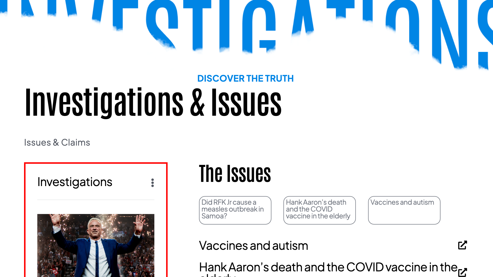
BSI Is excited to release our Investigation section of the Broken Science web site. This page features investigative work we've been doing in the background.
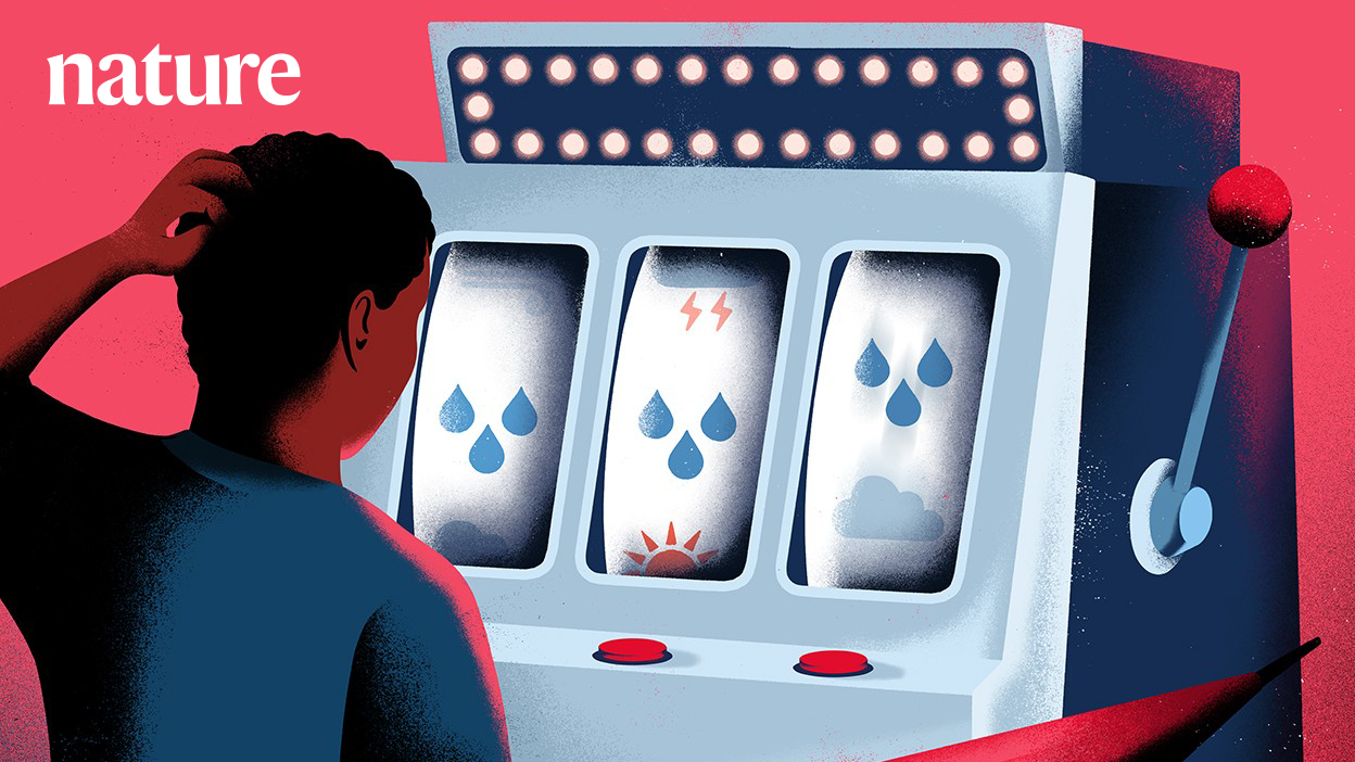
All of statistics and much of science depends on probability — an astonishing achievement, considering no one’s really sure what it is.